本文从零实现一个大模型,用于帮助理解大模型的基本原理,本文是一个读书笔记,内容来自于Build a Large Language Model (From Scratch)
目录 本系列包含以以下主题,当前在主题三
1. 文本处理 2. 注意力机制 4. 使用无标记数据预训练模型 5. 分类微调 6. 指令微调 上一章内容实现了注意力机制,注意力机制的目标是生成上下文向量,这一章的会开发类GPT-2的模型类
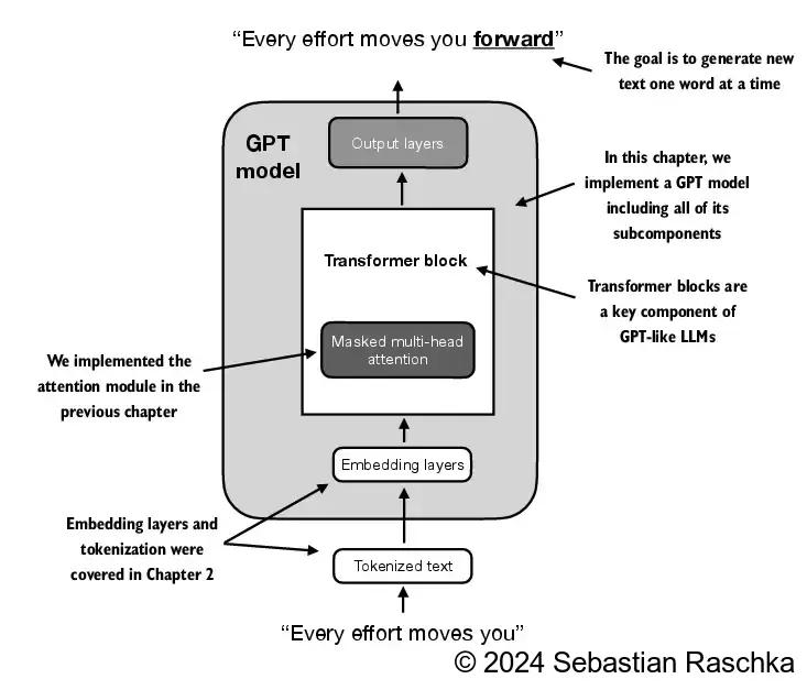
构建模型 类GPT模型的架构图如下,该类主要包含以下两个个未实现的模块:Output layers和Transformer block。其他模块在之前的章节中已经实现。
首先初始化GPTModel类所需的配置参数
1
2
3
4
5
6
7
8
9
GPT_CONFIG_124M = { "vocab_size" : 50257 , "context_length" : 1024 , "emb_dim" : 768 , "n_heads" : 12 , "n_layers" : 12 , "drop_rate" : 0.1 , "qkv_bias" : False }
模型类的的代码结构如下
1
2
3
4
5
6
7
8
9
10
11
12
13
14
15
16
17
18
19
20
21
22
23
24
25
26
27
28
29
30
31
32
33
34
35
36
37
38
39
40
41
42
43
44
45
46
47
48
49
50
import torchimport torch.nn as nnclass DummyGPTModel (nn.Module): def __init__ (self, cfg ): super ().__init__() self.tok_emb = nn.Embedding(cfg["vocab_size" ], cfg["emb_dim" ]) self.pos_emb = nn.Embedding(cfg["context_length" ], cfg["emb_dim" ]) self.drop_emb = nn.Dropout(cfg["drop_rate" ]) self.trf_blocks = nn.Sequential( *[DummyTransformerBlock(cfg) for _ in range (cfg["n_layers" ])]) self.final_norm = DummyLayerNorm(cfg["emb_dim" ]) self.out_head = nn.Linear( cfg["emb_dim" ], cfg["vocab_size" ], bias=False ) def forward (self, in_idx ): batch_size, seq_len = in_idx.shape tok_embeds = self.tok_emb(in_idx) pos_embeds = self.pos_emb(torch.arange(seq_len, device=in_idx.device)) x = tok_embeds + pos_embeds x = self.drop_emb(x) x = self.trf_blocks(x) x = self.final_norm(x) logits = self.out_head(x) return logits class DummyTransformerBlock (nn.Module): def __init__ (self, cfg ): super ().__init__() def forward (self, x ): return x class DummyLayerNorm (nn.Module): def __init__ (self, normalized_shape, eps=1e-5 ): super ().__init__() def forward (self, x ): return x
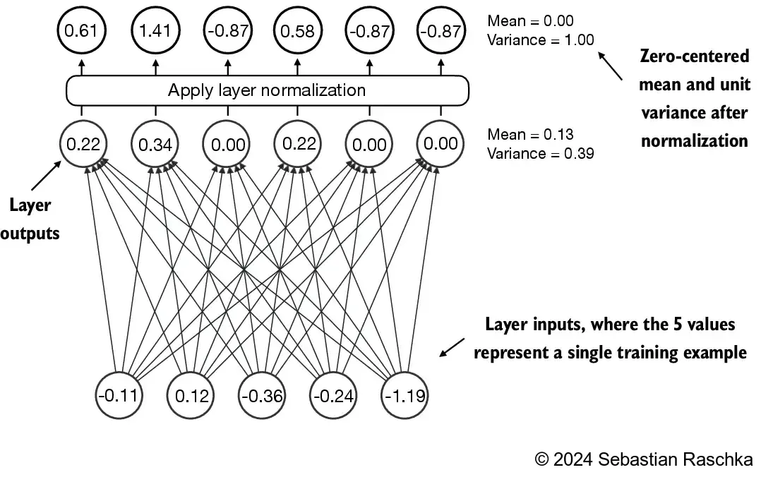
归一化层 首先需要实现的的归一化层,即上文代码中的LayerNorm,该类的作用是将inputs的最后一个维度(嵌入向量的维度,emb_dim)进行标准化,将他们的值调整为均值为 0,方差为 1(即单位方差)。
梯度指的是变化率,描述了某个值(例如函数输出值)对另一个值(如输入变量)的变化趋势。大模型在应用梯度的概念时,首先会设计一个损失函数,用来衡量模型的预测结果与目标结果的差距。在训练过程中,它通过梯度去帮助每个模型参数不断调整来快速减少损失函数的值,从而提高模型的预测精度。
上图演示了一个具有5个输入和6个输出的神经网络层,输出层的6个值,其均值为0,方差为1。
1 2 3 4 5 6 7 8 9 10 11 12 13 14 15 16 17 18 19 20 21 22 23 24 torch.manual_seed(123 ) batch_example = torch.randn(2 , 5 ) layer = nn.Sequential(nn.Linear(5 , 6 ), nn.ReLU()) out = layer(batch_example) print (out)mean = out.mean(dim=-1 , keepdim=True ) var = out.var(dim=-1 , keepdim=True ) print ("Mean:\n" , mean)print ("Variance:\n" , var)print ("\n" )out_norm = (out - mean) / torch.sqrt(var) mean = out_norm.mean(dim=-1 , keepdim=True ) var = out_norm.var(dim=-1 , keepdim=True ) print ("Normalized layer outputs:\n" , out_norm)print ("Mean:\n" , mean)print ("Variance:\n" , var)
tensor([[0.2260, 0.3470, 0.0000, 0.2216, 0.0000, 0.0000],
        [0.2133, 0.2394, 0.0000, 0.5198, 0.3297, 0.0000]],
       grad_fn=<ReluBackward0>)
Mean:
 tensor([[0.1324],
        [0.2170]], grad_fn=<MeanBackward1>)
Variance:
 tensor([[0.0231],
        [0.0398]], grad_fn=<VarBackward0>)


Normalized layer outputs:
 tensor([[ 0.6159,  1.4126, -0.8719,  0.5872, -0.8719, -0.8719],
        [-0.0189,  0.1121, -1.0876,  1.5173,  0.5647, -1.0876]],
       grad_fn=<DivBackward0>)
Mean:
 tensor([[-5.9605e-08],
        [ 1.9868e-08]], grad_fn=<MeanBackward1>)
Variance:
 tensor([[1.0000],
        [1.0000]], grad_fn=<VarBackward0>)
以上是层归一化的实现原理,根据以上过程,LayerNorm的具体实现如下:
1
2
3
4
5
6
7
8
9
10
11
12
13
14
class LayerNorm (nn.Module): def __init__ (self, emb_dim ): super ().__init__() self.eps = 1e-5 self.scale = nn.Parameter(torch.ones(emb_dim)) self.shift = nn.Parameter(torch.zeros(emb_dim)) def forward (self, x ): mean = x.mean(dim=-1 , keepdim=True ) var = x.var(dim=-1 , keepdim=True , unbiased=False ) norm_x = (x - mean) / torch.sqrt(var + self.eps) return self.scale * norm_x + self.shift
调用上面的层归一化类
1
2
3
4
5
6
ln = LayerNorm(emb_dim=5 ) out_ln = ln(batch_example) mean = out_ln.mean(dim=-1 , keepdim=True ) var = out_ln.var(dim=-1 , unbiased=False , keepdim=True ) print ("Mean:\n" , mean)print ("Variance:\n" , var)
Mean:
 tensor([[-2.9802e-08],
        [ 0.0000e+00]], grad_fn=<MeanBackward1>)
Variance:
 tensor([[1.0000],
        [1.0000]], grad_fn=<VarBackward0>)
使用GELU激活函数实现前馈神经网络 接下来需要实现一个前馈神经网络FeedForward类,但是在实现这个类之前要先了解一下GELU激活函数,GELU激活函数是更复杂、平滑的激活函数,分别结合了高斯分布和 sigmoid 门控线性单元。他可以为深度学习模型提供更好的性能。这里暂时不深究他的数学原理,直接实现:
1
2
3
4
5
6
7
8
9
class GELU (nn.Module): def __init__ (self ): super ().__init__() def forward (self, x ): return 0.5 * x * (1 + torch.tanh( torch.sqrt(torch.tensor(2.0 / torch.pi)) * (x + 0.044715 * torch.pow (x, 3 )) ))
实现了GELU激活函数之后,就可以实现前馈神经网络了,FeedForward 模块是一个小型神经网络,由两个线性层和一个 GELU 激活函数组成
1
2
3
4
5
6
7
8
9
10
11
class FeedForward (nn.Module): def __init__ (self, cfg ): super ().__init__() self.layers = nn.Sequential( nn.Linear(cfg["emb_dim" ], 4 * cfg["emb_dim" ]), GELU(), nn.Linear(4 * cfg["emb_dim" ], cfg["emb_dim" ]), ) def forward (self, x ): return self.layers(x)
前馈神经网络的输入和输出具有相同的维度
1
2
3
4
5
6
ffn = FeedForward(GPT_CONFIG_124M) x = torch.rand(2 , 3 , 768 ) out = ffn(x) print (out.shape)
torch.Size([2, 3, 768])
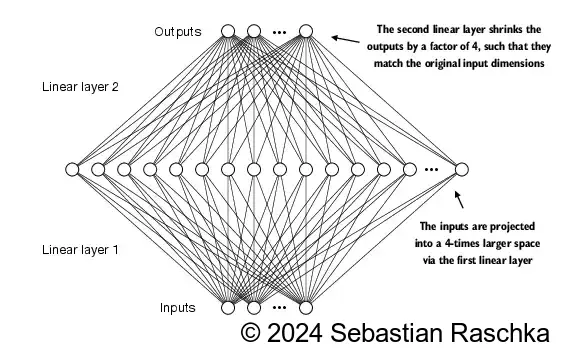
这里实现的 FeedForward 模块对模型能力的增强(主要体现在从数据中学习模式并泛化方面)起到了关键作用。尽管该模块的输入和输出维度相同,但在内部,它首先通过第一个线性层将嵌入维度扩展到一个更高维度的空间。之后再接入非线性 GELU 激活,最后再通过第二个线性层变换回原始维度。这样的设计能够探索更丰富的表示空间。上面的架构如图所示
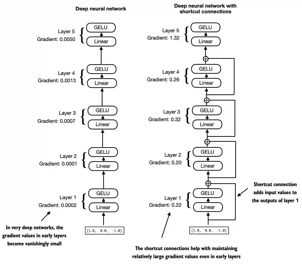
实现快捷连接 接下来,还要再讨论一下快捷连接(也称跳跃连接或残差连接)的概念,它用于缓解梯度消失问题。梯度消失是指在训练中指导权重更新的梯度在反向传播过程中逐渐减小,导致早期层(靠近输入端的网络层)难以有效训练。
简单的说,快捷连接有以下两个作用:
保持信息(或者说是特征)流畅传递
缓解梯度消失问题
快捷连接的实现示例如下
1
2
3
4
5
6
7
8
9
10
11
12
13
14
15
16
17
18
19
20
21
22
class ExampleDeepNeuralNetwork (nn.Module): def __init__ (self, layer_sizes, use_shortcut ): super ().__init__() self.use_shortcut = use_shortcut self.layers = nn.ModuleList([ nn.Sequential(nn.Linear(layer_sizes[0 ], layer_sizes[1 ]), GELU()), nn.Sequential(nn.Linear(layer_sizes[1 ], layer_sizes[2 ]), GELU()), nn.Sequential(nn.Linear(layer_sizes[2 ], layer_sizes[3 ]), GELU()), nn.Sequential(nn.Linear(layer_sizes[3 ], layer_sizes[4 ]), GELU()), nn.Sequential(nn.Linear(layer_sizes[4 ], layer_sizes[5 ]), GELU()) ]) def forward (self, x ): for layer in self.layers: layer_output = layer(x) if self.use_shortcut and x.shape == layer_output.shape: x = x + layer_output else : x = layer_output return x
接下来实现一个函数打印梯度对比观察使用快捷连接的效果
1
2
3
4
5
6
7
8
9
10
11
12
13
14
15
16
17
def print_gradients (model, x ): output = model(x) target = torch.tensor([[0. ]]) loss = nn.MSELoss() loss = loss(output, target) loss.backward() for name, param in model.named_parameters(): if 'weight' in name: print (f"{name} has gradient mean of {param.grad.abs ().mean().item()} " )
不使用快捷连接时的结果如下:
1
2
3
4
5
6
7
8
9
layer_sizes = [3 , 3 , 3 , 3 , 3 , 1 ] sample_input = torch.tensor([[1. , 0. , -1. ]]) torch.manual_seed(123 ) model_without_shortcut = ExampleDeepNeuralNetwork( layer_sizes, use_shortcut=False ) print_gradients(model_without_shortcut, sample_input)
layers.0.0.weight has gradient mean of 0.00020173587836325169
layers.1.0.weight has gradient mean of 0.0001201116101583466
layers.2.0.weight has gradient mean of 0.0007152041071094573
layers.3.0.weight has gradient mean of 0.0013988735154271126
layers.4.0.weight has gradient mean of 0.005049645435065031
梯度在从最后一层(layers.4)到第一层(layers.0)时逐渐减小,这种现象称为梯度消失问题。再看看使用快捷连接的效果:
1 2 3 4 5 torch.manual_seed(123 ) model_with_shortcut = ExampleDeepNeuralNetwork( layer_sizes, use_shortcut=True ) print_gradients(model_with_shortcut, sample_input)
layers.0.0.weight has gradient mean of 0.22169791162014008
layers.1.0.weight has gradient mean of 0.20694106817245483
layers.2.0.weight has gradient mean of 0.32896995544433594
layers.3.0.weight has gradient mean of 0.2665732204914093
layers.4.0.weight has gradient mean of 1.3258540630340576
可以已经没有梯度消失的问题了。
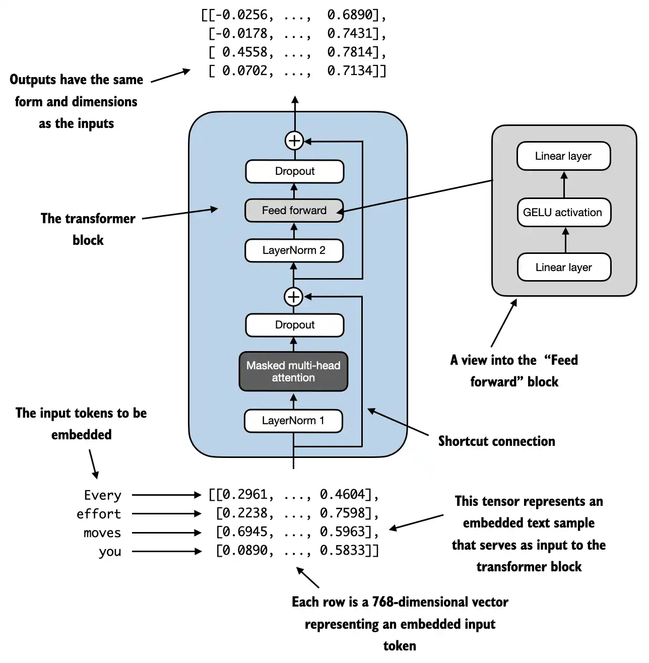
以上模块实现之后,接下来就可以实现GPTModel类的核心模块TransformerBlock类了,他的结构图如下
根据上面的架构图,将之前实现的子模块组装成TransformerBlock类
1
2
3
4
5
6
7
8
9
10
11
12
13
14
15
16
17
18
19
20
21
22
23
24
25
26
27
28
29
30
31
32
33
from gpt import MultiHeadAttention class TransformerBlock (nn.Module): def __init__ (self, cfg ): super ().__init__() self.att = MultiHeadAttention( d_in=cfg["emb_dim" ], d_out=cfg["emb_dim" ], context_length=cfg["context_length" ], num_heads=cfg["n_heads" ], dropout=cfg["drop_rate" ], qkv_bias=cfg["qkv_bias" ]) self.ff = FeedForward(cfg) self.norm1 = LayerNorm(cfg["emb_dim" ]) self.norm2 = LayerNorm(cfg["emb_dim" ]) self.drop_shortcut = nn.Dropout(cfg["drop_rate" ]) def forward (self, x ): shortcut = x x = self.norm1(x) x = self.att(x) x = self.drop_shortcut(x) x = x + shortcut shortcut = x x = self.norm2(x) x = self.ff(x) x = self.drop_shortcut(x) x = x + shortcut return x
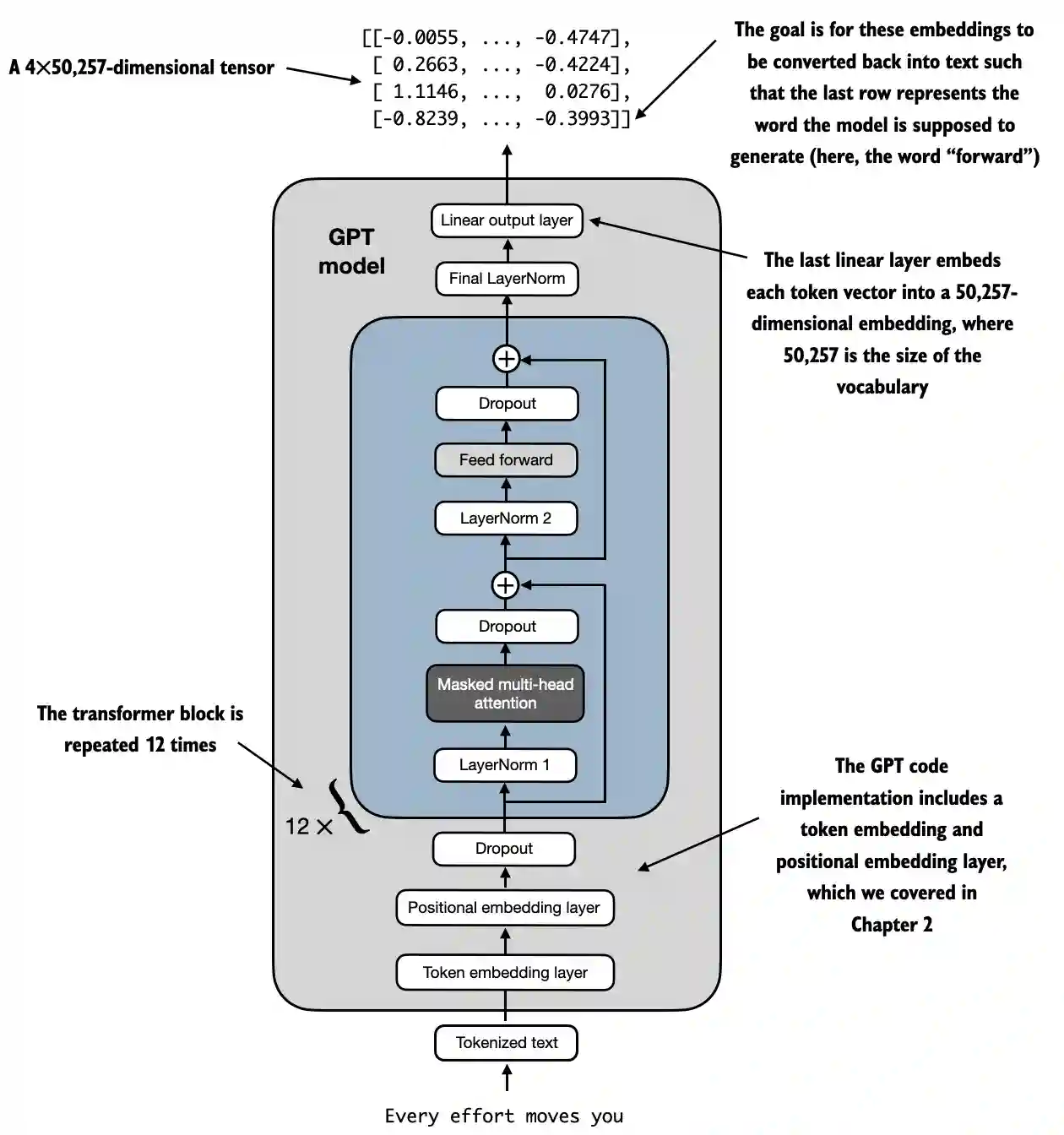
实现GPTModel类 核心模块TransformerBlock类实现之后,就可以实现GPTModel类了,类架构图如下:
根据上面的架构图,将之前实现的函数组装成GPTModel类
1
2
3
4
5
6
7
8
9
10
11
12
13
14
15
16
17
18
19
20
21
22
23
24
25
26
class GPTModel (nn.Module): def __init__ (self, cfg ): super ().__init__() self.tok_emb = nn.Embedding(cfg["vocab_size" ], cfg["emb_dim" ]) self.pos_emb = nn.Embedding(cfg["context_length" ], cfg["emb_dim" ]) self.drop_emb = nn.Dropout(cfg["drop_rate" ]) self.trf_blocks = nn.Sequential( *[TransformerBlock(cfg) for _ in range (cfg["n_layers" ])]) self.final_norm = LayerNorm(cfg["emb_dim" ]) self.out_head = nn.Linear( cfg["emb_dim" ], cfg["vocab_size" ], bias=False ) def forward (self, in_idx ): batch_size, seq_len = in_idx.shape tok_embeds = self.tok_emb(in_idx) pos_embeds = self.pos_emb(torch.arange(seq_len, device=in_idx.device)) x = tok_embeds + pos_embeds x = self.drop_emb(x) x = self.trf_blocks(x) x = self.final_norm(x) logits = self.out_head(x) return logits
文本测试 创建一个辅助函数测试上面的GPTModel类
1
2
3
4
5
6
7
8
9
10
11
12
13
14
15
16
17
18
19
20
21
22
23
24
25
26
27
def generate_text_simple (model, idx, max_new_tokens, context_size ): for _ in range (max_new_tokens): idx_cond = idx[:, -context_size:] with torch.no_grad(): logits = model(idx_cond) logits = logits[:, -1 , :] probas = torch.softmax(logits, dim=-1 ) idx_next = torch.argmax(probas, dim=-1 , keepdim=True ) idx = torch.cat((idx, idx_next), dim=1 ) return idx
1
2
3
4
5
6
7
8
9
10
11
12
13
14
15
16
17
18
19
20
21
22
23
24
25
26
27
28
29
import tiktokentorch.manual_seed(123 ) model = GPTModel(GPT_CONFIG_124M) model.eval () start_context = "Hello, I am" tokenizer = tiktoken.get_encoding("gpt2" ) encoded = tokenizer.encode(start_context) encoded_tensor = torch.tensor(encoded).unsqueeze(0 ) print (f"\n{50 *'=' } \n{22 *' ' } IN\n{50 *'=' } " )print ("\nInput text:" , start_context)print ("Encoded input text:" , encoded)print ("encoded_tensor.shape:" , encoded_tensor.shape)out = generate_text_simple( model=model, idx=encoded_tensor, max_new_tokens=10 , context_size=GPT_CONFIG_124M["context_length" ] ) decoded_text = tokenizer.decode(out.squeeze(0 ).tolist()) print (f"\n\n{50 *'=' } \n{22 *' ' } OUT\n{50 *'=' } " )print ("\nOutput:" , out)print ("Output length:" , len (out[0 ]))print ("Output text:" , decoded_text)
可以看到,经过模型处理后,已经有输出了,但是输出的内容还是错误的,这是因为模型还没有经过任何的训练,下一章要训练模型,来输出合理的内容。